How to lock cells to Excel in formulas
When you compose a formula on Excel, in almost all cases you use cell references to automatically acquire the data already present in the sheet. If the formula has to be repeated several times, the operation that you surely put into practice is to drag the cell that contains it into those below or adjacent to it.
By carrying out this procedure, however, what happens is that the reference of the rows or columns of a cell is translated. Although in some cases this consequence can be useful, in others there is the risk of creating errors in the calculation of the formulas, especially for those that repeat themselves but have static values taken from a single cell or from a specific range.
To solve this drawback, it is necessary lock cells in formulas, so that their references cannot in any way be translated. This operation is possible only by entering the $ symbol within the cell reference. Let's see in detail how to do it.
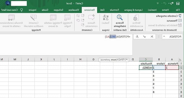
Let's take the cell as an example C2, inside which the simple formula was typed = POWER (B2: A2) (to calculate the power of a value equal to A2 on the number present in B2).
In the column B you therefore have a series of values on which to calculate the power and in the column C you need to repeat the formula as many times as there are values in B. By dragging the formula down, the cell B2 contained in the formula would be replaced with B3, then with B4 and so on, so that the cell reference follows the values in the table in column B. As for A2instead, dragging would cause the cell reference to be transformed into A3 and progressive, with the consequent error in the formula as the value is present only in A2.
To fix this, you simply need to transform the cell A2 in $ A $ 2, prefixing the $ symbol on both the column reference and the row reference. You can also edit the formula and place the typing pointer on the cell and press the key F4 repeatedly, until complete blockage occurs, as I have indicated to you. Once the cell is locked, any horizontal or vertical dragging will leave the cell reference unchanged in subsequent formulas.
Another case that can occur is when you need to block the reference of only the column or row of a cell. In this case, the procedure to follow is similar to the one I showed you in the previous paragraphs: affix the $ symbol on the column reference (ex. $ A2) or on that of the line (eg. A $ 2) to lock the column or row of a cell respectively within the formula.
The consequences of what I have illustrated to you are the following: in the event that you have blocked the column (eg $ A2), in case of horizontal dragging of the formula the reference will remain on column A, but by dragging the formula vertically the row reference will change (e.g. $ A3, $ A4, etc.). If you have blocked the line (ex. A $ 2), if the formula is dragged vertically the reference will remain on row 1, but by dragging the formula horizontally the column reference will change (e.g. B $ 3, C $ 4, etc.).
How to freeze cells in Excel scrolling
When working in Excel with a large amount of data, it is often necessary that some cells, such as those relating to the column header, are locked during scrolling, so as to avoid going back to the beginning of the sheet to understand each column. what you are referring to.
To perform this operation, you must proceed by carefully following the instructions that you will find in the next chapters, in which I will show you in detail how lock cells in Excel while scrolling both on the classic version of the program for Windows and macOS and in its Web version and in the Excel app for smartphones and tablets.
Microsoft Excel (Windows/macOS)
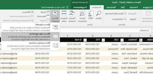
In Microsoft Excel for Windows and macOS you can freeze cells of a row or column via the feature Freeze Panes. All you have to do to make use of it is to reach the tab Show and press the button Freeze Panes, to view the available options.
Selecting the voice Freeze Top Row, the first row of the sheet will be locked while choosing Freeze first column, you will keep the locked view of the first column of the sheet. The option Freeze Panes, on the other hand, it allows you to freeze multiple rows or multiple columns, unlike the other two options I told you about, which are limited only to the first row / column of the sheet.
To use the latter feature, select the row or column next to the range you want to block and press the option Freeze Panes, to confirm the display lock. To clarify, if you want to block the range of lines A1: A3, you need to select the whole row A4 and then click on the option Freeze Panes.
Excel Online (Web)
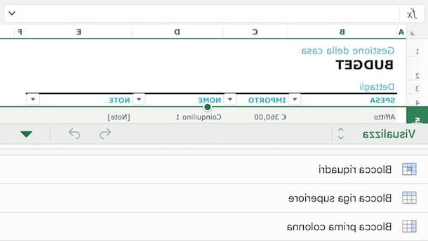
If you are using the web version of Excel, you can easily perform the freeze panes operation using the same functionality found in the Microsoft Excel desktop client. Via the tool Freeze Panes present in the menu Show, you can freeze the first line (Freeze Top Row) or the first column (Freeze first column).
Furthermore, you can also freeze a range of rows or columns, using the option Freeze Panes. For the operation of this feature, you can refer to what I indicated in the previous chapter.
Office (Android / iOS / iPadOS)
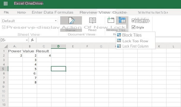
The app was used Office for Android and iOS or the app Excel for Android and iOS / iPadOS, you can freeze cell display while scrolling in a quick and easy way. As I described to you in the chapters relating to the desktop client and the web version of Microsoft Excel, even in the variants of Excel for mobile devices it is possible to do this through the functionality Freeze Panes.
All you have to do is reach for the tab Show, available in the top section on a tablet or in the drop-down menu at the bottom of a smartphone. Once this is done, click on the item Freeze Panes and choose one of the three available options: Freeze Panes, Freeze Top Row e Freeze first column, which I have told you about in detail in this chapter.
How to lock cells in Excel with password
If you need to share an Excel document and you don't want some cells to be changed or the formulas contained in them can be readable, what you need to do is protect the document with a Password. I warn you, however, that this procedure is only possible on the client desktop di Microsoft Excel and therefore you will not be able to act either from the Excel web platform or from the app for smartphones and tablets.
To create a protected Excel workbook, what you need to do is, first, locate the cells you want to block. By default, all cells are set to be automatically locked as soon as a password is set.
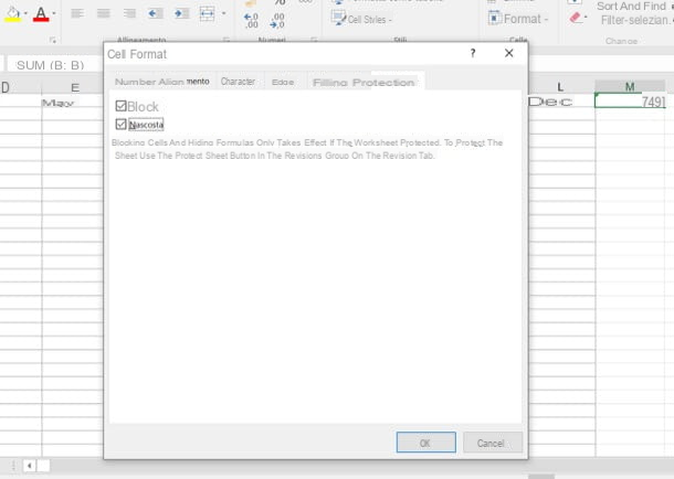
First, select the cell or range of cells you want to lock a cell on or hide the formula it contains. Once this is done, right click on the highlighted area and choose the item Celle format give the menu answer.
At this point, in the screen that is shown to you, reach the tab Protection and activate the box Blocked, to make sure that its content cannot be changed, then put a check mark on Hidden, to not allow you to view the formula inside but only the result that is generated.
Now, go to the tab revision, click the icon Protect sheet and, in the box that is shown to you, enter the Password. Then make sure there is a check mark in the box Protect worksheet and contents of locked cells. All you have to do is press the button OK and re-enter the Password previously indicated, to confirm the operation.
If you want to know more about how to protect cells in an Excel workbook, you can check out what I have explained to you in detail in my guide on how to protect cells in Excel.
How to lock cells in Excel