How to freeze an Excel row on PC
Do you want to know how to freeze an Excel row on PC, via the classic desktop software for Windows and macOS or via the Excel Online web service? In this case, you just have to read carefully the procedures that I will show you in the next chapters and put them into practice.
Freeze the first row of an Excel sheet
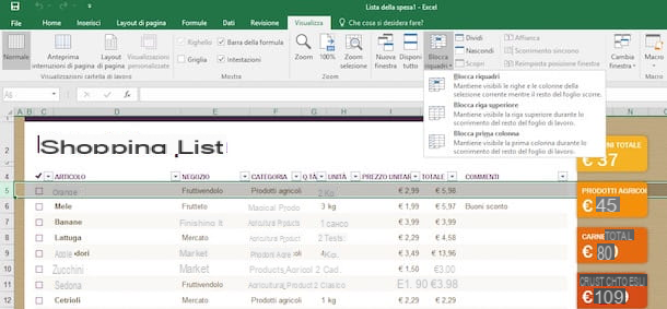
If you need to freeze the first row of your spreadsheet so that you can see the headings of a table, all you have to do is go to the tab Show toolbar Excel (above), click on the button Freeze Panes located on the right and select the item Freeze Top Row give the menu check if you press.
This way, even if you scroll down the document, the contents of the first row will remain fixed at the top of the screen allowing you to see the headings of the table.
You don't want to block the first line, you want to block the first column of an Excel sheet? No problem, this function is also available in Excel. All you have to do is select the tab Show (above), click on the button Freeze Panes (top right) and choose the item Freeze first column give the menu to compare.
This way, while scrolling the worksheet horizontally, the first column of values will remain frozen and always visible on top.
Freeze multiple rows of an Excel sheet
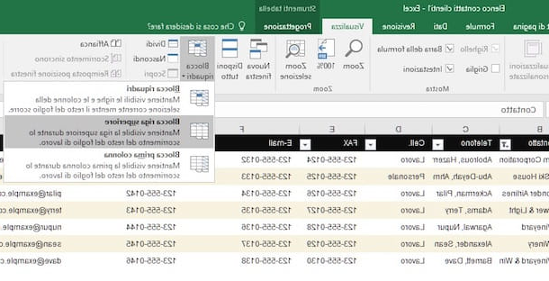
Excel also allows you to freeze a set of sequential lines (that is, which come one after the other), just select the line immediately following those to be fixed and activate the option Freeze Panes from the program menu.
Let's take a practical example: let's say you want to block therow range from 1 to 5. The first operation you need to do is to select the row number 6 (by clicking on the number 6 beside the Excel sheet).
Then go to the card Show Excel (top), click on the button Freeze Panes and select the item Freeze Panes from the menu that appears. Easy, right? This procedure can also be performed on column, following in principle the same indications that I have given you in the previous paragraphs.
Freeze rows and columns
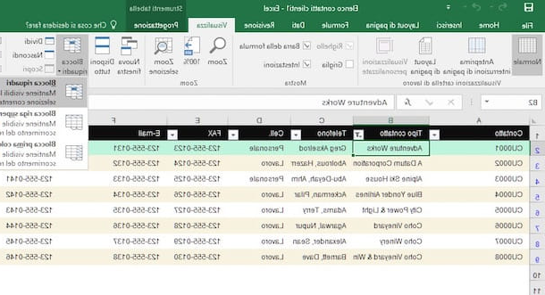
Using the same function that I described to you in the previous chapter, you can also freeze rows and columns at the same time. Just select the cell located immediately below and immediately to the right of the range of rows and columns to be "fixed". Let's take another practical example to better understand the topic.
If you have a table with (riga 1) the titles of the various columns and in the first column (A) the names of the customers, it might be useful to block both and keep them always visible.
To get this result, you need to select the cell first B2, which is immediately to the right of the column to be blocked and immediately below the row to be blocked. Then go to the card Showclick on your bottone Freeze Panes and select the item Freeze Panes give the menu to compare.
When you have finished your work on the spreadsheet, to unlock the rows and columns set for "fixed" view, go back to the tab Show Excel, click on the button Freeze Panes and select the item Unfreeze Panes give the menu to compare.
How to block an Excel row on smartphones and tablets
As you surely know, Excel it is also available as an app for Android (also downloadable from alternative stores) and iOS / iPadOS. It is free for devices with displays equal to or less than 10,1 inches in size (otherwise it requires a subscription to Microsoft 365, starting at 7 euros / month) and even in this mobile incarnation it allows you to block the rows and columns of the spreadsheets. Let's see immediately how.
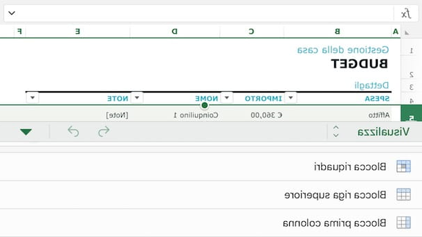
First, select a row or column by tapping on the respective label. Later, if you use Excel from tablet, select the scheda Show (top) and presses the button Freeze Panes. Excel is used to smartphoneinstead, tap the drop down menu located at the bottom left and select the items View> Freeze Panes da quest'ultimo.
At this point, you have several options to choose from: Freeze Panes to freeze the selected rows or columns, Freeze Top Row to lock only the first row of the sheet or Freeze first column to lock only the first column of the sheet.
To lock both rows and columns simultaneously, you can follow the same instructions I gave you in the previous chapter. Therefore, select the cell and then press on the items View> Freeze Panes> Freeze Panes, to carry out the operation.
When you are done working, you can unlock the rows and columns of the spreadsheet by pressing the button Freeze Panes Excel and removing the check mark from the option activated above. The procedure applies to both smartphones and tablets.
How to freeze Excel row in print
You are in a situation where you have a spreadsheet with a lot of data spread over numerous lines. At the time of printing, however, the data is reported on the sheet, losing the column headings, although you have blocked the top row, as I have already explained to you in the previous chapters?
To solve this problem and, therefore, make sure that the labels of the columns in the first row are repeated on all printed pages, you must follow the procedures that I will show you in the next rows, which can only be implemented on the classic Excel for Windows and macOS.
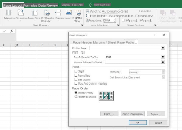
To proceed, select the tab Layout on the pagina that you find at the top and press the button Print titlesIn section Set page. In the screen that is shown to you, then click on the card Sheet and click the button with the up arrow che trovi to fianco della dicitura Lines to repeat at the top.
At this point, click on the line number and press again onarrow icon, this time facing down. If the data to be repeated on the printout concerns several lines, select all the necessary ones. Finally, press on the button OK to confirm.
I warn you that this operation can also be useful for fixing some columns on the printout: the procedure is identical to the one I indicated in the previous paragraphs, but you will have to act on the item Columns to repeat on the left.
Now, pressing on the items File> Print you can see the print preview and, as you scroll through the pages, you will notice how the rows and / or columns you have selected are repeated on each page.
How to freeze Excel dollar row
When you insert cell references in a formula and then proceed to repeat the latter in all cells by dragging, these references are inevitably incremented.
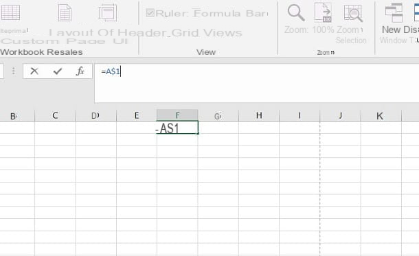
For example, in the cell F1 the expression = A1 is indicated and, by dragging vertically, in the following cells the expressions become = A2, = A3 and so on.
If your interest is to fix the cell reference so that it does not vary in any way when expressions are reported on other cells, what you need to do is freeze the row with the dollar symbol (works in any version of Excel).
To do this, all you have to do is enter the dollar symbol between the letter and number that distinguishes the cell reference. Therefore, considering the above example, for cell reference A1, you will need to write the expression = A $ 1.
This way, even if you drag the formula, the cell reference row will be locked. If you then add the dollar symbol even before the letter (= $ A $ 1), you will also block the column.
How to freeze an Excel row